Normative Modelling
Normative modelling provides an opportunity to quantify departures from the typical population
using statistical regression techniques. This technique can be useful in neuroimaging
since it could be the degree of deviation from typical peers that is predictive of function
rather than the raw metric value itself. Normative modelling can also be useful when studying
development in children and adolescents given that there can be varying trajectories among children.
An added complexity is that neuroimaging metrics change over the course of development as children mature.
Normative modelling allows researchers to embrace individual variability along a developmental trajectory
while at the same time identifying possible deviations from that trajectory that may be clinically informative.
Multimodal Neuroimaging
Magnetic resonance (MR) imaging provides a unique opportunity to measure brain characteristics in many different ways.
- Cortical morphometry captures structural information such as the thickness of the grey matter
ribbon (cortical thickness) in atlas-based regions of interest or volumes of grey matter structures.
- Functional connectivity captures how fluctuations in blood oxygenation levels vary over time
(at rest) and how synchronous these temporal patterns can be in spatially separate but
related regions of the brain, inferring that those areas are functionally connected.
- Diffusion imaging can capture information about the underlying microstructure of white matter,
possibly informing us on how well these bundles transmit information between brain areas.
In the FIDELITI Dashboard, these neuroimaging metrics are in turn grouped within broader functional domains of
interest. These domains include sensorimotor, language, vision, attention, memory, and
audition. The result is that over 150 neuroimaging features are available for viewing in
the dashboard.
Reference Cohort
A large reference cohort of children, adolescents, and young adults is available for comparison.
Approximately 900 control participants with no neurological conditions ranging in age from 5-22 years
compose the reference cohort. This cross-sectional cohort defines the range of typical variability
on over 150 extracted neuroimaging features. These individuals were scanned on 3T scanners as part
of the Human Connectome Project (Development) or at the Alberta Children’s Hospital, a tertiary
care hospital with a research-dedicated scanner. Imaging from this cohort has been processed using
the same pipelines that will process your participants allowing for meaningful comparisons.
Dashboard Workflow
FIDELITI has a simple workflow. First, participants' demographic information and imaging session files
are entered. Processing pipeline(s) are then selected according to which neuroimaging modalities
are available. Once processing has been successfully completed, the desired functional domain profile can be selected
and the dashboard can be viewed.
Security and Privacy
To ensure security and privacy of sensitive data, the demographic and imaging data you enter
into the FIDELITI Dashboard never leave your local computer. Data is not transmitted at any time to any
online cloud-based servers. For additional privacy, potentially sensitive demographic
information such as dates of birth or names are not required and names can be changed
(or omitted) if preferred. Participants can be tracked through the Dashboard solely through
their anonymized ID number. Note also that all names shown in this documentation have been
changed to ensure privacy and confidentiality.
Dependencies
In order for the full multimodal analysis pipelines to be operational, the FIDELITI Dashboard
requires several other software packages to be installed. Note that if you already have these
installed on your system, these steps can be skipped.
- MATLAB Runtime Library R2017b (9.3). This runtime library is
required for the cortical morphometry (CAT12) standalone processing toolbox and does not
require a MATLAB license. This library should be installed within this folder:
/Applications/MATLAB/Matlab_Runtime/v93. If it is installed elsewhere on your computer please specify where it
is installed using the FIDELITI Preferences page.
- MATLAB Runtime Library R2021a (9.10). This runtime library is
required for the functional connectivity (CONN) standalone processing toolbox and does
not require a MATLAB license. This library should be installed within this folder:
/Applications/MATLAB/Matlab_Runtime/v910. If it is installed elsewhere on your computer please specify where it
is installed using the FIDELITI Preferences page
- The FMRIB Software Library (FSL)
is a powerful imaging software that is required for the white matter microstructure
processing pipeline. FSL can be installed using the default settings.
- MRtrix3 is an advanced
white matter imaging tool that is required for the white matter microstructure pipeline and
for certain quality assessment tools. MRtrix3 can be installed using the default settings.
Checking Installation
To check that the dependencies have been correctly installed, you can navigate to the
Preferences page and click the Check Installation button. This will check whether
FIDELITI can access FSL, MRtrix3, and the MATLAB Runtime Libraries successfully.
If the dependencies have been successfully installed (or were installed previously),
you should see four green checkboxes in this area.
If there are errors, please try to reinstall the applicable dependency and click
the check installation button again.
Preference Settings
When first starting out with the FIDELITI Dashboard, a few preferences need to be specified. Please see the
Preferences section for more details.
- FIDELITI working folder - This is the folder where the processed imaging files will be
saved on your system. By default, this is set to: /Desktop/FIDELITI. It can be updated in
Preferences.
- MATLAB Runtime folder - Several toolboxes require the MATLAB Runtime libraries. By
default they are installed to /Applications/MATLAB/MATLAB_Runtime. However, if you have the
folders for v93 and v910 installed in a different folder, that folder needs to be specified
in Preferences.
Running FIDELITI
Once you have successfully installed the Dashboard and all the dependencies, you can simply double click
the FIDELITI icon in your Applications folder to open it.
The first page you will see upon opening the Dashboard is the Home screen. This contains useful
information for users first starting with FIDELITI. The navigation wizard in the top right corner
can help to point out the next (and previous) steps in the work flow. Or you can work your way down
the navigation menu on the left side of the main window.
Participant Demographics
To manually enter a participant session, click the Add Session button. To copy a session,
click on the session to copy and click the Copy Session button. This can be helpful for
entering several sessions for the same participant. To delete a session, click on the session
to be deleted and click the Delete Session button. Any changes must be saved by clicking the
Save Changes button. The Reload List button can be used to
discard any unwanted changes and revert to the previously saved list.
The five mandatory fields are indicated with bold column headings. Demographics can be entered by clicking in each table cell and entering
the applicable information. Note that cells are yellow when in editing mode and blue when in selection mode.
- ID - Participant ID (mandatory). Consider this ID the unique identifier for each
participant that will identify them throughout the Dashboard. If a participant has multiple
sessions (i.e., for a longitudinal study), the ID should be entered on multiple lines
corresponding to each session but must be exactly the same for the data to be grouped
properly on graphs and reports. If you prefer to keep all sessions separate for a given
participant, then a suffix denoting the session can be added to the ID number to keep them
unique. For example, S01-T1, S01-T2, S01-T3. Note that when entered this way, these sessions
will be treated as unique participants and multiple session data points will not be displayed on the same graph.
- First Name and Last Name (optional) - These fields are not required, they are included
only for your reference. Names can be changed for anonymization purposes. Note that names entered
here will appear on Dashboard summary reports.
- Sex (mandatory) - This is the biological sex of the participant and is entered as
M (male) or F (female). Sex is mandatory here for best accuracy because the normative models
are stratified by sex. If you prefer to enter gender instead (i.e., if sex and gender are
different for a given participant), the gender should also be entered using M (male) or F (female).
- Age (mandatory) - Age is entered in years. Please ensure that this age is as close
to the actual age at scanning (if it needs to be altered for anonymization purposes). Currently,
children, adolescents, and young adults between the ages of 5.5 and 22.0 years can be accommodated in the Dashboard. As
additional data is added in future releases, this age range may expand.
- Project (optional) - Project is not required, it has been included only for your reference.
This field can be helpful for grouping when sorting your participant table.
- Session Date (optional) - The date of the imaging session is not mandatory and is
included here for your reference. This field can be helpful when working with longitudinal data.
- Session (mandatory) - The Session Description is mandatory since it is used in the
folder structure during processing to organize files. This description will also appear on the
Dashboard reports. Please do not use spaces or special characters in this description.
Note that any changes made to the information in this table needs to be saved using the
Save Changes button before moving on to the next steps.
Imaging Files
Imaging files can be entered here by clicking in the applicable cell and selecting the
corresponding file in nifti format (*.nii). Note that this file should be unzipped. This
means that files with the extension *.nii.gz should be converted to *.nii before importing. This is
easily done by double-clicking the zipped (*.nii.gz) in your Finder.
- T1 - T1-weighted image (mandatory) - This single file is a high-resolution T1-weighted anatomical image.
The T1-weighted image is mandatory for all pipelines since it is a central part of pre-processing.
For best results, a resolution of 1 mm isotropic is best if possible. This file will also be used
in the cortical morphometry pipeline for extracting cortical thickess measurements and grey matter volumes.
- RS - Resting State fMRI images (optional) - This single file is a 4-dimensional resting
state functional MRI file that has beeen acquired while the participant was at rest or watching
a relaxing visual display. For best results, this file should contain at least 100 volumes, more
volumes if possible. This file is mandatory if using the resting state functional connectivity
pipeline.
- DW - Diffusion-weighted images (optional) - This single file is a 4-dimensional
diffusion-weighted imaging file containing at least six diffusion gradients, more if possible.
A single pair of *.bval and *.bvec files that define the gradient directions should be in FSL
format and should be located in the same directory. Note that the names of these bval and bvec
files do not matter, they just are required to have the file extensions .bval and .bvec.
Note that any changes made to the information in this table needs to be saved using the
Save Changes button before moving on to the next steps.
Dicom to Nifti Conversion
If your imaging files are in dicom format (common when first extracted from the scanner),
they can be converted to nifti format here. First make sure the dicoms are organized into
separate folders (by sequence), then click one of the conversion buttons to select the folder.
The newly created nifti file will be named anat.nii, rs.nii, or dwi.nii according to the sequence and will
be saved in the dicom directory originally selected. This new *.nii file can then be selected
in the participant session list above for further processing.
Importing Multiple Participants
If you have an entire cohort of participants to enter, it can be helpful to use the batch
import functionality. This will require a *.csv file containing the demographic information
for each participant as well as the complete path to their imaging files. Once this file is
selected using the Select Import file button, the participants will be added to the participant
session list above. Make sure you click the Save Changes button to save your new participant
session list, or click the Reload List button to discard any changes.
The *.csv file must contain all column headings, however only the data for the mandatory
fields need to be entered.
Note that the Save Changes button needs to be clicked
after importing a cohort to save the additions to the participant session table before moving on to the next steps.
Processing Queue
The Processing Queue is a listing of the sessions you
wish to process. First, select a participant session in the Participant list on the left
side and using the rightward arrow button, add it to the To be processed listing (i.e., the processing queue). This
should be repeated for all sessions to be processed. Then click Save Changes. Multiple
sessions can be selected and added to the processing queue at the same time.
Note that selecting participants with the same available imaging files for the same batch is helpful here
(scroll to the right on either table to view which imaging files are available). For example,
selecting a participant with a missing diffusion file alongside others with diffusion files will
cause a "file missing" error when you select the diffusion pipeline in the next step. Instead,
choose the participants with the same set of imaging to be processed in a single batch. Then,
once that batch has been submitted for processing, construct a new batch of participants with
matching imaging files to be submitted next.
Subsequent batches can be submitted before the
previous batches are finished processing and will be queued accordingly. Sessions will be processed
in parallel depending on your system resources though if the batches are larger, some sessions will be processed serially.
At this stage, please ensure that every participant session contains the mandatory
information required (ID, Sex, Age, Session, T1 image). Note that this participant list is read only.
To update participant information, return to the Participant page, update the information,
save the changes and return to this page. If your participant does not appear in this listing, return
to the Participants page and make sure that they have been successfully entered there and that
all changes have been saved. Then return to this page. Your participant information should now appear here.
To remove a participant session from the "To be processed" list, select the session and click the
leftward arrow to remove it. To clear the entire processing queue, click Clear Queue. Click Save Changes.
Note that the Save Changes button needs to be clicked
after constructing or changing your "To be processed" list before moving on to the processing preferences step.
Processing Preferences
Once the Processing Queue has been constructed, the desired pipelines can be selected. Note
that the Cortical Morphometry pipeline requires a high-resolution T1-weighted image. The
Functional Connectivity pipeline requires a high-resolution T1-weighted image AND a
4-dimensional resting state image containing at least 100 volumes. The White matter microstructure
pipeline requires a high-resolution T1-weighted image AND a diffusion-weighted image containing at
least six diffusion directions. Once you have selected the desired pipelines, click Run Processing
to start the processing. Processing proceeds in the background and you can still use the Dashboard
while this processing proceeds.
If you close the Dashboard before the image processing is
complete, processing will stop. Note that unsaved changes will be lost. You may also need to close
the MATLAB runtime application separately to stop all processing.
Cortical Morphometry
The Cortical Morphometry pipeline uses the Computational Anatomy Toolbox
(CAT12) for Statistical Parametric Mapping (SPM) running in Matlab to calculate cortical
morphometry metrics such as cortical thickness within atlas-based regions of interest and grey matter
volumes for various structures. More information about CAT12 can be found here: CAT12
Functional Connectivity
The functional connectivity pipeline uses the Connectivity Toolbox (CONN)
for SPM running within Matlab to calculate temporal cross correlations in fluctuations in blood
oxygen-level dependent (BOLD) response between regions of interest across the brain. Brain regions are
defined using the Harvard-Oxford Atlas and their functional connectivity is quantified using
Fisher-transformed Pearson correlation coefficients.
White Matter Microstructure
The white matter microstructure pipeline uses functions from MRtrix3
and FSL to calculate
fractional anisotropy across the brain to quantify the diffusion of water within white matter
structures of interest. These structures are defined via regions from the Johns
Hopkins University (JHU) White Matter Atlas.
Custom Pipelines
If you would like to add participants that have already been pre-processed (perhaps with your own
customized processing pipeline), this functionality exists though is for advanced users. It is easiest
to start with existing datafiles from other pre-processed participants to make sure the formatting
and column headings are correct.
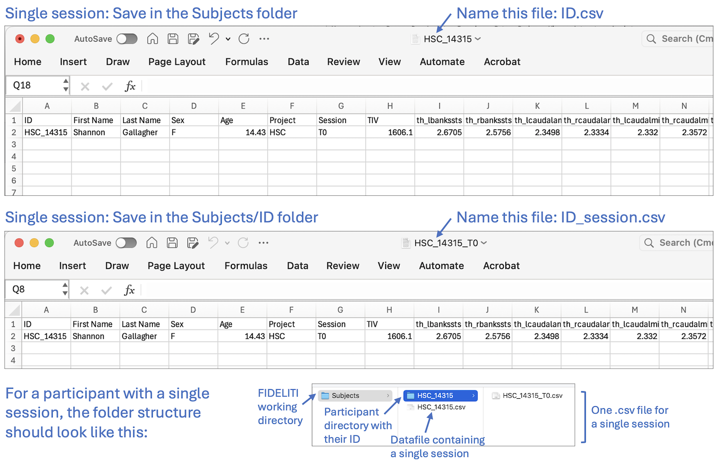
- Single session - Prepare your participants’ datafile containing cortical morphometry,
functional connectivity, and/or white matter microstructure
feature values in a single row in the format provided above (with all column names that match those existing in FIDELITI).
Save this file as a comma delimited .csv file in the Subjects folder of your working directory.
This working directory is specified in the FIDELITI Preferences page. The
datafile must be named with your participant ID (ID.csv). Then, within the Subjects folder, create a participant folder with their ID.
Within this folder (Subjects/ID), save the same data file with the name ID_session.csv. Click on the first example
image above for an illustration.
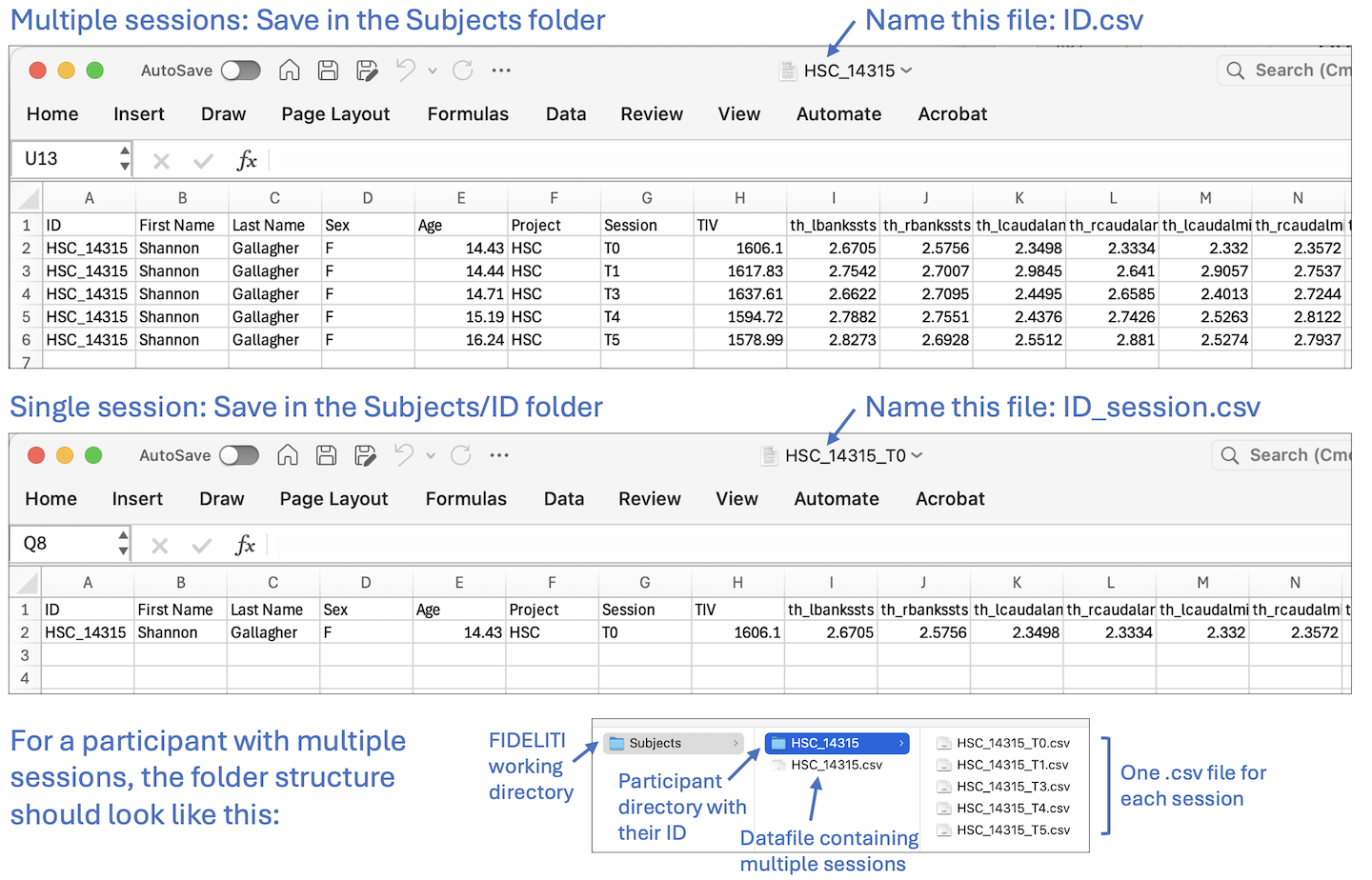
- Multiple sessions - Prepare your participants’ datafile containing cortical morphometry,
functional connectivity, and/or white matter microstructure
feature values for each session in their own row in the format provided above (with all column names that match those existing in FIDELITI).
Save this file as a comma delimited .csv file in the Subjects folder of your working directory.
This working directory is specified in the FIDELITI Preferences page. The
datafile must be named with your participant ID (ID.csv). Then, within the Subjects folder, create a participant folder with their ID.
Within this folder (Subjects/ID), save one data file per session each with only one row of data. Name these files ID_session.csv. Click on the second example
image above for an illustration.
Once you have completed these steps, open FIDELITI and you should be able to select
and view your participant’s Dashboard in the Dashboard tab. We recommend using pipelines that
are similar to the ones supplied with the FIDELITI Dashboard to minimise differences between
your participants and the normative database that may be introduced by different processing pipelines.
For a complete listing of column
names (case-sensitive) that are required please refer to the Neuroimaging Feature List
or Supplementary Table 1 from Carlson et al (2026). All column headings (features) need to be included even if there is
no data associated with them. Note that the order of the feature columns does not need to conform
to the order given here except for the first seven demographic columns. For longitudinal data,
include multiple rows where each row corresponds to an imaging session (and the session name and age changes accordingly).
Note that if the custom pre-processing pipeline differs too
much from the processing that has been done on the control data, then this will introduce systematic biases
in the deviation scores. For best results, use a similar processing pipeline as that used for the controls.
Neuroimaging Feature List
A full list of neuroimaging features is available in the Supplementary section Neuroimaging Feature List.
Participant Session and Profile Selection
A listing of available participants and sessions is displayed on this page. Participants are
sorted by ID in this listing and have additional demographic information listed for your reference.
To view the Dashboard for a single participant session, locate your participant in the list,
roll down the arrow to expand the session list and click on the session of interest. Then select
the profile you would like to view (i.e., the functional domain) on the right side and click the View Dashboard
button just below. The Dashboard for that participant session and functional domain
will be displayed below. Click on the left example above for an illustration.
For participants with multiple sessions, you can view features for all sessions on the same
graph for comparison across time. Simply select the parent record above the multiple
sessions, select the functional profile of interest, and click View Dashboard. For example,
if a participant has five imaging sessions that have been successfully processed, then five
red symbols should be displayed on each graph. Click on the centre example above for an illustration.
If your participant only has partial data, for example has only been successfully processed through
the cortical morphometry pipeline, then the graphs for other features for functional connectivity
and white matter microstructure will still show blue and purple
symbols but will not have red symbols. You will also see nan (not a number) instead of deviation
scores in the top left corner of each graph that has missing data. These can just be disregarded.
Click on the right example above for an illustration.
FIDELITI Graphs
FIDELITI Dashboard graphs are rich in information.
- Title - The graph title contains the region(s) of interest that are being displayed in the graph.
These regions are determined by the various atlases that were defined during pre-processing.
For example, R PostCG is the postcentral gyrus in the right hemisphere. For functional connectivity,
there are two regions in the title which represent the two regions between which the connectivity
has been calculated. For example, R PreCG - R Caudate represents the functional connectivity between
the right precentral gyrus and the right caudate. For a complete listing of all features with descriptions,
please see the Neuroimaging Feature List in the supplementary information section.
- Y-axis - The y-axis defines the neuroimaging feature and its native units. This will be
one of functional connectivity (units: rF Fisher-transformed Pearson correlation coefficient), grey matter volume (units: cm3),
cortical thickness (units: mm), or fractional anisotropy (white matter microstructure).
- X-axis - The x-axis is the age in years. Your participant will be plotted using the age
that was entered in the participant list. It is important to have this age as close as possible to
the participant's actual age at scanning (if it needs to be altered for anonymity) for maximal accuracy
of plotting and deviation score calculations.
- Symbols - The purple circles (females) and blue squares (males) on the graphs represent feature values for
a cross-sectional sample of typically developing controls. These symbols illustrate the trajectory of the feature values
across the age range and the two distributions are stratified by biological sex.
- Regression lines - Regression lines are fit using a piecewise regression function via
locally estimated scatterplot smoothing (LOESS) calculated using the control data points for
females (purple) and males (blue) separately. Shaded areas represent the 95% confidence intervals
around each line of best fit.
- Deviation scores - Deviation scores define departures (residuals) between actual and predicted
feature scores and are expressed in native feature units (d), as z-scores (standard deviations (SD)
from the mean), and as percentiles based on the sex and age of the participant. For example, a
cortical thickness deviation (d) score is expressed in millimeters, and a functional connectivity
deviation score is expressed as a Fisher-transformed Pearson correlation coefficient. By contrast,
z-scores of both are expressed in SD from the mean of the distribution, and percentiles are expressed
as the proportion of scores falling below the participant’s feature score. If a participant has
multiple sessions, the deviation scores represent only the first session (i.e., the youngest age).
User-defined thresholds for displaying
these values in red can be specified in Preferences. More
information on how to export deviation scores can be found in the
Export Deviation Scores section. Note that if these deviation
scores appear as "nan" (not a number), this indicates that this participant does not have successfully
processed data for this neuroimaging feature. For example, if no diffusion imaging is available, the
white matter microstructure graphs will not have any red symbols and will have "nan" displayed for deviation scores for the
white matter graphs but red symbols and deviation scores may be present for the other cortical thickness, grey matter volume, and functional
connectivity graphs. If your participant's age is out of the range within which deviation scores can be calculated,
you will see a red "range" error in place of the deviation scores. Please check that your participant has an age between 6-22 years.
- Participant results - Results for the current participant are displayed using red symbols
where the shape reflects the sex (circle - female, square - male). The range of the
y-axis will auto-calculate to accommodate a wide range of participant feature values. For a single imaging session,
just one red symbol will be displayed. For multiple sessions, more than one red symbol each representing one time point will be displayed.
If the imaging sessions were performed when the participant was of similar ages, there may be overlap
between the symbols. If no symbols are displayed, this may indicate missing data. Check in the participant
folder to see if the processing has completed correctly.
Summary Report
A PDF version of a participant's Dashboard can be saved in the form of a Summary Report by clicking the View
Summary Report button. Just as in the Dashboard, if a single session is selected in the session listing,
only that single session will be included in the Summary Report. If the master participant record is
selected, all sessions will be included in the report. Also, the profile you currently have selected
will be used to generate the report. Once viewing the report, save it using the File/Save as
menu option in your PDF viewer. Note that reports are not automatically saved to preserve space on your system and will
be overwritten each time the View Summary Report button is pressed unless each one is manually saved to
another location.
Export Deviation Scores
Deviation scores can be exported to a .csv file for later analysis by clicking the Export Deviation
Scores button. If you have selected a single session, the deviation scores for that session will
be saved to that session folder for your participant. If you are clicked on the master record for your
participant, all deviation scores for all sessions will be saved to each of the session folders for your
participant. Note that the functional domain (profile) currently selected is ignored and all deviation scores
for all neuroimaging features are included in these files. The files are saved separately for each type of deviation score, and
which types of deviation scores that are saved when you click this button can be specified in Preferences.
- d scores - filename: ID_session_d.csv
- z scores - filename: ID_session_z.csv
- Percentiles - filename: ID_session_pct.csv
Quality Assessment
Quality checking the image processing is a very important step. There are multiple methods provided in the Dashboard.
- View Anatomy - The View anatomy button will display the original T1-weighted anatomical
image that was entered in the participant list. This image opens with MRview, an image viewer that is
part of the MRtrix3 package. Please ensure you have
installed MRtrix3 to use this functionality. Navigate
around the T1 image by clicking, zooming, and using the menu options. More information can be found in the
MRtrix3 documentation.
- Check Cortical Morphometry - This button will open the CAT12 report that resulted from
processing data through the cortical morphometry pipeline which contains useful image quality and tissue segmentation information.
For more information on the CAT12 report please see their documentation.
This report can also be found in the Subjects/participant/session/CAT12/report folder.
- Check Functional Connectivity - The Check Functional Connectivity button opens a carpet plot
illustrating head motion before and after denoising. This image is generated by the CONN toolbox and contains
useful information on head motion and outliers that may affect data quality. For more information on CONN,
see their documentation here.
This image can also be found in the
Subjects/participant/session/CONN/FIDELITI_FC/results/qa folder along with an image illustrating
the quality of the normalization process.
- Check White Matter - The Check White Matter button opens an MRview window with the participant's
fractional anisotropy (FA) map displayed. MRview is part of the MRTrix3 package so ensure you have MRtrix3 installed on your system.
Overlaid on the FA map are the warped JHU white matter regions of
interest that have been used to extract the median FA value for each region. Diffusion scans are inherently
lower resolution than the high-resolution T1-weighted images and so this image may appear "blocky". Use the
Tool/ROI editor to view the names of the ROIs displayed.
Profile List
The Profile List contains a listing of all profiles that are currently available in the Dashboard.
To add a new profile, select an existing profile and click Duplicate Selected Profile. Enter the name
and description of the new Profile then click Save Changes. You can then scroll down to the Profile
Edit area to edit the neuroimaging features that are displayed in the profile when viewing the Dashboard.
If you prefer to start from a blank profile, click the Add Blank Profile button instead, enter
the new name and description, and click Save Changes. To delete an existing profile, select the profile you wish to
delete and click Delete Profile. The Save Changes button must be clicked for any profile list changes to be saved.
Note that the Save Changes button needs to be clicked when
any changes are made to the profiles listing for those changes to be saved.
Profile Edit
To change the contents of a profile, first select it in the Profile List. Then edit the neuroimaging
features you wish to appear within that profile. When finished editing, click the Save Profile Changes
button.
Having a profile with too many neuroimaging features can
become unwieldy. It is best to have smaller numbers of features in multiple profiles.
MATLAB Runtime Directory
The cortical morphometry and functional connectivity pipelines both use toolboxes that require
MATLAB Runtime to be installed (no MATLAB License is required). By default, the MATLAB Runtime libraries are installed
in the folder: /Applications/MATLAB/MATLAB_Runtime.
However, if you have the folders for v93 and v910 installed in a different folder, that folder needs
to be specified here. Click the Select Directory button to specify the MATLAB Runtime folder. Then click
Save Preferences.
FIDELITI Working Directory
During image processing, the Dashboard needs to save processed files and summary results to a folder
on your system. By default, this is Desktop/FIDELITI. If you would like your participants' processed
imaging folders and data files to be saved somewhere else, please click the Select Directory button
and select this folder here. Then click Save Preferences.
Deviation Score Settings
Deviation score thresholds determine the value at which z-score and percentile values are displayed
in red on each dashboard graph. For example, setting a lower z-score threshold of -3.1 would display
a red z-score for any values lower than 3.1 standard deviations below the mean and black z-scores
for other values that do not exceed this threshold (e.g., z=-2.4). For percentiles, the threshold defines the
percentile point under which the percentile value is displayed in red (e.g., 15th percentile).
If you prefer to not use thresholds (and keep the deviation scores always displayed in black), uncheck the
Use deviation score thresholds box.
Export deviation scores checkboxes specify which deviation scores will be exported (as .csv files)
if you wish to perform further processing using these values. If these
checkboxes are all checked, then clicking the Export Deviation Scores button on the Dashboard page will
save three .csv files to the FIDELITI working directory (specified above) /Subjects/ID/session
folder. For example, by default these files would be saved to: /Desktop/FIDELITI/Subjects/ID/session.
- d scores - filename: ID_session_d.csv
- z-scores - filename: ID_session_z.csv
- percentiles - filename: ID_session_pct.csv
Resting State fMRI Settings
Resting state processing settings can be specified here. Specifically the repetition time (TR) in seconds,
the smoothing kernel in mm, and the slice timing correction setting (drop down list). Note that these
settings should be set for your data before the processing starts.
Scanner Harmonization
Harmonization procedures attempt to reduce the effects of different scanners and sequences in
multi-site data by statistically transforming one dataset to more closely resemble a reference
dataset while at the same time conserving individual biological variability. The FIDELITI Dashboard uses
Neurocombat to harmonize between the scanners. For more information on how this was done, please
refer to Carlson et al (2026). For more information on Neurocombat, please see
Fortin et al. (2017)
and neuroCombat.
The Alberta Children's Hospital (ACH) scanner is a 3T GE MR750w, similar to scanners found in research settings.
The Human Connectome Project - Development (HCD) scanners are 3T Siemens Prisma scanners customized
for the HCD Project. We recommend that you choose the option where the reference most closely resembles
your scanner and scanning protocol. The default is to use the ACH scanner as the reference since it
may be closer to a typical research scanner found in hospital and university settings, however other
options are available.
Note that the deviation scores will change for every participant and every
neuroimaging feature if the harmonization option is changed so be sure to select the desired option
before you analyze your data. If you need to update it after you have processed your imaging, you can
simply export all the deviation scores again for each participant and the value in the new .csv files will
reflect deviation scores based on the new harmonized distributions.
Main Log
The main log listing contains information about viewing different participant dashboards. It may also
contain error messages resulting from an inability to load certain files. The main log can be copied into
another application of your choice or it can be saved as a text file. You can also clear the contents of the
log if you wish.
Job Listing
The job listing area contains individual logs for each currently running job and for previously completed jobs. For example,
if a cortical morphometry pipeline is currently running, progress messages will be streamed to a job area
reflecting the current process. If a functional connectivity job is also submitted, a new job area will appear
that contains progress messages for that job. Jobs can be cancelled while running. All job logs can also be copied
for transfer into another application or can be saved to a text file. Logs can also be cleared if desired.
Installation
Do I need a MATLAB Licence?
No MATLAB license is required though two MATLAB Runtime libraries are required for full functionality.
Please see the Installation Dependencies documentation for information
on the MATLAB Runtime libraries required (v93 and v910). Also see the Preference Settings for
information on how to specify the MATLAB Runtime Library folder.
Do I need both MATLAB Runtime Libraries or can I just install one?
Both MATLAB Runtime libraries are required for full pipeline functionality. Specifically, version v93 is
required for the cortical morphometry (CAT12) processing pipeline and version v910 is required for
the functional connectivity (CONN) pipeline. If either are missing, you will not be able to run
these pipelines on your participant. Please see the Dependencies
documentation for information.
How do I know that installation of dependencies has been successful?
To check that the dependencies are correctly installed and are accessible to the Dashboard, please access
the Preferences page and click the Check Installation button. If the dependencies are all successfully installed,
you should see four green checkmarks in this area. For more information, please see Checking Installation
documentation.
Processing
Why does my participant session not appear in the Participant list on the Processing page?
If your participant does not appear in this listing, return to the Participants page and make sure
that your participant has been successfully entered there and that all changes have been saved. Then return
to the Processing page to work with the participant.
Why can’t I edit my participant in the processing queue?
Note that the participant list in the Processing page is read only. To update participant information,
return to the Participants page, update the information, save the changes, and return to the Processing page.
Can I submit more than one batch to the processing queue?
Yes more than one batch can be submitted at the same time. Choosing participants with the same set of imaging to be processed
in a single batch is helpful to avoid errors. Then, once that batch has been submitted for processing,
construct a new batch of participants with matching imaging files to be submitted next. Subsequent
batches can be submitted before the previous batches are finished processing and will be queued
accordingly depending on your system capabilities.
Can I run more than one participant/pipeline at the same time?
Yes, you can run more than one participant session and more than one imaging modality pipeline at the same time.
This is typically done in batches via the Processing page. Depending on your system, the jobs will
run in parallel where possible. Therefore, you may see multiple MATLAB applications open in the background
at the same time. Running too many jobs at the same time will degrade your system’s performance
for other tasks and so we recommend not running too many participants and sessions at the same time (e.g., <10 sessions).
Can I do other things within the dashboard while pipeline processing is running?
Yes, you can navigate around the Dashboard and view other pages while the processing is running.
You can also prepare and submit other batches for processing which will be queued accordingly depending
on the capacity of your system.
I closed the Dashboard main window while processing was running, will it still finish?
If the Dashboard main window is closed during processing, processing will stop. Note that all unsaved changes will be lost.
Please reopen the Dashboard and restart the processing if it does not complete correctly. You can
still navigate around inside the Dashboard while the processing is running, just do not close the
Dashboard application window. Minimizing the main FIDELITI window while processing participant data is also fine,
processing will continue.
How do I know when data processing is finished?
When the data processing is completed, your participant will have an ID.csv file in their Subjects folder
within the working directory on your computer (check where this working directory is in
the Preferences page)
and will also be selectable in the list menu on the Dashboard page of FIDELITI. If your participant
does not appear in this list and processing has completed, click the Refresh List button. If they still do not appear, check
that all applicable imaging files were correctly specified in the Participants page and that there
are no errors in the log areas.
Why do I get the error: Image is not in NIFTI-1.1 format?
Please ensure that all your *.nii files have been unzipped, i.e., they are not in *.nii.gz format.
This can typically be done in MacOS by double-clicking the file in Finder to unzip. Then re-enter
the file into the Participants page.
If I re-run the same participant with the same ID and session, will my previous results be overwritten?
Yes, if you use the same ID and session the previous results will be overwritten.
Dashboard
Why does my participant not appear in the Dashboard list?
If your participant does not appear in the Dashboard list, it could be that the processing is not yet complete.
Try clicking the Refresh List button. If they still do not appear, this usually means that no
processing has been successfully completed for them or it is still processing. Please return to the Participants page and
ensure that the appropriate imaging files are specified for your participant and that they have been saved.
Then proceed to the Processing page, delete and re-add your participant to the “to be processed” queue,
select your pipeline(s) of choice with the checkboxes at the bottom, and click “Run Processing”.
Once the processing has successfully finished, return to the Dashboard page and click the Refresh
List button and your participant should now appear in the dashboard listing.
In my participant’s Dashboard, why are there no red symbols in some of the graphs?
If you do not see your participant’s data in their dashboard (i.e., there are no red symbols on some
of the graphs), that usually means that either your participant has no imaging feature data for that modality
(i.e., a missing imaging file), or the processing for that imaging modality has not yet been completed.
Please check that you have processed your participant’s data through that pipeline (functional connectivity,
cortical morphometry, white matter microstructure) and then access the dashboard page again.
How are the regression lines in the Dashboard graphs calculated?
The regression lines are calculated using a LOESS regression model (locally estimated scatterplot smoothing).
A LOESS model uses a least-squares regression to locally fit a smooth curve through complex data
without making any assumptions as to the underlying data distribution. This means that the LOESS
model is non-parametric therefore robust to outliers and also allows the calculation of confidence
intervals around the mean. Each of the two regression lines (purple - female, blue - male) are
calculated using feature values from the reference cohort based on age and sex. For more information on
the regression calculations, please see Carlson et al. (2026).
What do the numbers represent in the upper left corner of the Dashboard graphs?
There are three values in the upper left corner of each Dashboard graph.
- A d-score, or deviation score ,
is the difference between your participant’s score and the expected score from the regression line
calculated using age- and sex-matched control participants. This d-score is expressed in native neuroimaging
feature units. For example, for a 10.2 year-old male, if the expected value for functional connectivity
between right and left hippocampi is 0.65 and your participant has a FC value for 0.20 then their
deviation score is –0.45. The negative denotes that your participant’s score is lower than the expected
value for control participants. d-scores are expressed in y-variable units, for example, a d-score
of +1.2 for hippocampal volume means that your participant has a hippocampal volume that is 1.2 cm3
higher than the estimated group mean for age- and sex-matched typically developing peers.
- The second value is the deviation z-score expressed in standard deviations from the mean. For example, if a
participant has a positive z-score of 0.95 this means that they fall 0.95 standard deviations above
the expected value for their age and sex. If this value is negative, for example z=-1.27, it means
that the participant’s score falls 1.27 standard deviations below the expected value.
- The last value is a percentile score. This value expresses the proportion of scores in the normative cohort
that the current participant falls above if they were rank-ordered. For example, if the participant
has a functional connectivity percentile value of 37.9%, this means that their functional connectivity
value is higher than 37.9% of the typically developing sample.
Why is my participant’s d-score "nan"?
If you see a d=nan (not a number) in the top left corner of a graph, this typically means that there
is no data on which to calculate a deviation score for your participant., i.e., either the pipeline
has not successfully been completed successfuly or this participant has missing imaging files.
Please ensure that the applicable pipeline has been run successfully for your participant and
then reload their dashboard. If there is no imaging file corresponding to this modality then these
"nan" values can be disregarded.
Why is my participant’s d-score "range"?
If you see a red "range" error in the top left corner of a graph, this typically means that your
participant's age is outside the range for which deviation scores can be calculated. This range is
between 6-22 years depending on the sex of the participant and the neuroimaging feature chosen. If this occurs,
please check that your participant's age is correct and falls within this range. We anticipate that wider age ranges will be available
in the future.
Why do I get this error: Extrapolation not allowed with blending?
This error has likely occurred because your participant’s age is outside the range for our reference
cohort and extrapolation outside of this range has not been enabled. The reference cohort ranges
are detailed in Carlson et al (2026) for each sex and imaging modality but generally
participants must be between 6 and 22 years of age.
What output files and folders are saved during processing?
The FIDELITI Dashboard exports many files during processing, most of which conform to the output formats
for the CAT12 and CONN toolboxes. The main data files that are of interest and are also used for
the dashboard plots are listed below. Files are saved to a folder called Subjects in the
FIDELITI Working Directory specified in the Preferences page.
Some files are saved to the session folder within the participant folder if they are session-specific.
- ID.csv - This file is named using your participant ID number and contains
the neuroimaging feature values extracted for each successfully processed pipeline. For a participant
with a single session, this file will have one row of feautre values. For a participant with
multiple sessions, there will be multiple rows where each one corresponds to a session. Also
included is the demographic information that is used to plot the participant in the neuroimaging
feature graphs (ID, age, sex).
- session folders - Within the subject directory are session directories named using
the session descriptions entered in the Participants page. These directories contain the
original imaging files provided as well as the processed files.
- ID_session_CAT.csv - This file contains the cortical morphometry (CAT12) neuroimaging
feature values only for a single session and is found in the session directory.
- ID_session_CONN.csv - This file contains the functional connectivity (CONN) neuroimaging
feature values only for a single session and is found in the session directory.
- ID_session_WM.csv - This file contains the white matter microstructure neuroimaging
feature values only for a single session and is found in the session directory.
- CAT12, CONN, and WM folders found within the session folders contain processed files
from each participant.
- ID_session_d.csv - This file contains the deviation scores for all neuroimaging
feature values for a single session and is found in the session directory.
- ID_session_z.csv - This file contains the z-scores for all neuroimaging
feature values for a single session and is found in the session directory.
- ID_session_pct.csv - This file contains the percentile scores for all neuroimaging
feature values for a single session and is found in the session directory.
Note that these last three deviation score (ID_session_*.csv) files are only saved if they are checked in the
Deviation Score Settings on the Preferences page and if the Export Deviation Scores button has been clicked in the Dashboard page.
How to cite the FIDELITI Dashboard
If you wish to cite the FIDELITI Dashboard, please use the folowing information:
Carlson HL, Hassett JD, Hilderley AJ, Maiani M, Romanow N, Craig BT, Forkert N, Kirton A (2026).
Fingerprinting individual differences in lesion impact through imaging: The FIDELITI Dashboard,
a personalized dashboard for brain health.
Funding Sources
We thank the participants and families that volunteered to be control participants in this research.
The original development of the FIDELITI Dashboard was kindly supported by a Project grant from
the Cerebral Palsy Alliance Research Foundation. Additional funding for the expansion of the
project to longitudinal data was provided by the Heart and Stroke Foundation of Canada via a
Grant-in-Aid. We sincerely thank our funding sources for making this work possible.
Neuroimaging Feature List
A full list of neuroimaging features available within the FIDELITI Dashboard is below.
There are over 150 features available.
Features are sorted by functional domain and by imaging modality where FC - Functional
connectivity, GMV - grey matter volume, CT - cortical thickness, WM - white matter microstructure.
L - left hemisphere, R - right hemisphere, FA - fractional anisotropy, Fasc - fasciculus. This table is also available
in Carlson et al (2026) as Supplementary Table S1.
Sensorimotor Domain (30 features)
| Feature |
Feature Description |
Imaging Modality |
| RPreCG-LPreCG |
L Precentral gyrus – R Precentral gyrus |
FC |
| LPreCG-LPostCG |
L Precentral gyrus - L Postcentral gyrus |
FC |
| RPreCG-RPostCG |
R Precentral gyrus - R Postcentral gyrus |
FC |
| LPreCG-LSMA |
L Precentral gyrus - L Supplementary Motor Area |
FC |
| RPreCG-RSMA |
R Precentral gyrus - R Supplementary Motor Area |
FC |
| LPreCG-LThal |
L Precentral gyrus - L Thalamus |
FC |
| RPreCG-RThal |
R Precentral gyrus - R Thalamus |
FC |
| LPreCG-LPut |
L Precentral gyrus - L Putamen |
FC |
| RPreCG-RPut |
R Precentral gyrus - R Putamen |
FC |
| LPreCG-LCaud |
L Precentral gyrus - L Caudate |
FC |
| RPreCG-RCaud |
R Precentral gyrus - R Caudate |
FC |
| RPostCG-LPostCG |
L Postcentral gyrus - R Postcentral gyrus |
FC |
| LPostCG-LThal |
L Postcentral gyrus - L Thalamus |
FC |
| RPostCG-RThal |
R Postcentral gyrus - R Thalamus |
FC |
| gmv_lPrcG |
L Precentral gyrus |
GMV |
| gmv_rPrcG |
R Precentral gyrus |
GMV |
| gmv_lPoCG |
L Postcentral gyrus |
GMV |
| gmv_rPoCG |
R Postcentral gyrus |
GMV |
| gmv_lCau |
L Caudate |
GMV |
| gmv_rCau |
R Caudate |
GMV |
| gmv_lPut |
L Putamen |
GMV |
| gmv_rPut |
R Putamen |
GMV |
| gmvth_lVentral_Anterior |
L Ventral Anterior Thalamus |
GMV |
| gmvth_rVentral_Anterior |
R Ventral Anterior Thalamus |
GMV |
| th_lprecentral |
L Precentral gyrus |
CT |
| th_rprecentral |
R Precentral gyrus |
CT |
| th_lpostcentral |
L Postcentral gyrus |
CT |
| th_rpostcentral |
R Postcentral gyrus |
CT |
| wm_cst_l_fa |
L Corticospinal tract FA |
WM |
| wm_cst_r_fa |
R Corticospinal tract FA |
WM |
Language Domain (30 features)
| Feature |
Feature Description |
Imaging Modality |
| LANG_L_IFG-LANG_R_IFG |
L Inferior Frontal gyrus - R Inferior Frontal gyrus |
FC |
| LANG_L_IFG-LANG_L_pSTG |
L Inferior Frontal gyrus - L Posterior Superior Temporal gyrus |
FC |
| LANG_R_IFG-LANG_R_pSTG |
R Inferior Frontal gyrus - R Posterior Superior Temporal gyrus |
FC |
| LANG_L_pSTG-LANG_R_pSTG |
L Posterior Superior Temporal gyrus - R Posterior Superior Temporal gyrus |
FC |
| gmv_lInfFroG |
L Inferior Frontal gyrus |
GMV |
| gmv_rInfFroG |
R Inferior Frontal gyrus |
GMV |
| gmv_lSupTemG |
L Superior Temporal gyrus |
GMV |
| gmv_rSupTemG |
R Superior Temporal gyrus |
GMV |
| gmv_lMidTemG |
L Middle Temporal gyrus |
GMV |
| gmv_rMidTemG |
R Middle Temporal gyrus |
GMV |
| gmv_lInfTemG |
L Inferior Temporal gyrus |
GMV |
| gmv_rInfTemG |
R Inferior Temporal gyrus |
GMV |
| gmv_lSupMarG |
L Supramarginal gyrus |
GMV |
| gmv_rSupMarG |
R Supramarginal gyrus |
GMV |
| th_lparsopercularis |
L pars opercularis |
CT |
| th_rparsopercularis |
R pars opercularis |
CT |
| th_lparstriangularis |
L pars triangularis |
CT |
| th_rparstriangularis |
R pars triangularis |
CT |
| th_lparsorbitalis |
L pars orbitalis |
CT |
| th_rparsorbitalis |
R pars orbitalis |
CT |
| th_lsuperiortemporal |
L Superior Temporal gyrus |
CT |
| th_rsuperiortemporal |
R Superior Temporal gyrus |
CT |
| th_lmiddletemporal |
L Middle Temporal gyrus |
CT |
| th_rmiddletemporal |
R Middle Temporal gyrus |
CT |
| th_linferiortemporal |
L Inferior Temporal gyrus |
CT |
| th_rinferiortemporal |
R Inferior Temporal gyrus |
CT |
| th_lsupramarginal |
L Supramarginal gyrus |
CT |
| th_rsupramarginal |
R Supramarginal gyrus |
CT |
| wm_slf_l_fa |
L Superior Longitudinal Fasc. FA |
WM |
| wm_slf_r_fa |
R Superior Longitudinal Fasc. FA |
WM |
Vision Domain (31 features)
| Feature |
Feature Description |
Imaging Modality |
| VIS_Med-VIS_Occ |
Visual Network medial - Visual Network Occipital |
FC |
| VIS_Med-VIS_L_Lat |
Visual Network medial - L Visual Network lateral |
FC |
| VIS_Med-VIS_R_Lat |
Visual Network medial - R Visual Network lateral |
FC |
| VIS_Occ-VIS_L_Lat |
Visual Network Occipital - L Visual Network lateral |
FC |
| VIS_Occ-VIS_R_Lat |
Visual Network Occipital - R Visual Network lateral |
FC |
| VIS_L_Lat-VIS_R_Lat |
L Visual Network lateral - R Visual Network lateral |
FC |
| gmvth_lPulvinar |
L Pulvinar |
GMV |
| gmvth_rPulvinar |
R Pulvinar |
GMV |
| gmv_lLinG |
L Lingual gyrus |
GMV |
| gmv_rLinG |
R Lingual gyrus |
GMV |
| gmv_lFusG |
L Fusiform gyrus |
GMV |
| gmv_rFusG |
R Fusiform gyrus |
GMV |
| gmv_lSupOccG |
L Superior Occipital gyrus |
GMV |
| gmv_rSupOccG |
R Superior Occipital gyrus |
GMV |
| gmv_lMidOccG |
L Middle Occipital gyrus |
GMV |
| gmv_rMidOccG |
R Middle Occipital gyrus |
GMV |
| gmv_lInfOccG |
L Inferior Occipital gyrus |
GMV |
| gmv_rInfOccG |
R Inferior Occipital gyrus |
GMV |
| gmv_lCun |
L Cuneus |
GMV |
| gmv_rCun |
R Cuneus |
GMV |
| th_llingual |
L Lingual gyrus |
CT |
| th_rlingual |
R Lingual gyrus |
CT |
| th_lfusiform |
L Fusiform gyrus |
CT |
| th_rfusiform |
R Fusiform gyrus |
CT |
| th_llateraloccipital |
L Lateral Occipital gyrus |
CT |
| th_rlateraloccipital |
R Lateral Occipital gyrus |
CT |
| th_lcuneus |
L Cuneus |
CT |
| th_rcuneus |
R Cuneus |
CT |
| wm_ptr_l_fa |
L Posterior Thalamic Radiations FA |
WM |
| wm_ptr_r_fa |
R Posterior Thalamic Radiations FA |
WM |
| wm_ccsplenium_fa |
Splenium FA |
WM |
Attention and Executive Function Domain (33 features)
| Feature |
Feature Description |
Imaging Modality |
| FPN_L_LPFC-FPN_L_PPC |
Frontoparietal network L Lateral Prefrontal cortex - L Posterior Parietal cortex |
FC |
| FPN_L_LPFC-FPN_R_LPFC |
Frontoparietal network L Lateral Prefrontal cortex - R Lateral Prefrontal cortex |
FC |
| FPN_L_PPC-FPN_R_PPC |
Frontoparietal network L Posterior Parietal cortex - R Posterior Parietal cortex |
FC |
| FPN_R_LPFC-FPN_R_PPC |
Frontoparietal network L Lateral Prefrontal cortex - R Posterior Parietal cortex |
FC |
| DAN_L_FEF-DAN_R_FEF |
Dorsal Attention Network L Frontal Eye Field - R Frontal Eye Field |
FC |
| DAN_L_FEF-DAN_L_IPS |
Dorsal Attention Network L Frontal Eye Field - L Intraparietal sulcus |
FC |
| DAN_R_FEF-DAN_R_IPS |
Dorsal Attention Network R Frontal Eye Field - R Intraparietal sulcus |
FC |
| DAN_L_IPS-DAN_R_IPS |
Dorsal Attention Network L Intraparietal sulcus - R Intraparietal sulcus |
FC |
| gmvth_lMedio_Dorsal |
L Mediodorsal Thalamus |
GMV |
| gmvth_rMedio_Dorsal |
R Mediodorsal Thalamus |
GMV |
| gmv_lCinG |
L Cingulate gyrus |
GMV |
| gmv_rCinG |
R Cingulate gyrus |
GMV |
| gmv_lSupParG |
L Superior Parietal gyrus |
GMV |
| gmv_rSupParG |
R Superior Parietal gyrus |
GMV |
| gmv_lAngG |
L Angular gyrus |
GMV |
| gmv_rAngG |
R Angular gyrus |
GMV |
| gmv_lPCu |
L Precuneus |
GMV |
| gmv_rPCu |
R Precuneus |
GMV |
| th_lsuperiorfrontal |
L Superior Frontal gyrus |
CT |
| th_rsuperiorfrontal |
R Superior Frontal gyrus |
CT |
| th_lprecuneus |
L Precuneus |
CT |
| th_rprecuneus |
R Precuneus |
CT |
| th_lcaudalanteriorcingulate |
L Caudal Anterior Cingulate |
CT |
| th_rcaudalanteriorcingulate |
R Caudal Anterior Cingulate |
CT |
| th_lrostralanteriorcingulate |
L Rostral Anterior Cingulate |
CT |
| th_rrostralanteriorcingulate |
R Rostral Anterior Cingulate |
CT |
| th_lposteriorcingulate |
L Posterior Cingulate |
CT |
| th_rposteriorcingulate |
R Posterior Cingulate |
CT |
| th_lsuperiorparietal |
L Superior Parietal gyrus |
CT |
| th_rsuperiorparietal |
R Superior Parietal gyrus |
CT |
| wm_ccgenu_fa |
Genu FA |
WM |
| wm_acr_l_fa |
L Anterior Corona Radiata FA |
WM |
| wm_acr_r_fa |
R Anterior Corona Radiata FA |
WM |
Memory Domain (36 features)
| Feature |
Feature Description |
Imaging Modality |
| RHippocampus-LHippocampus |
L Hippocampus - R Hippocampus |
FC |
| LHippocampus-LAmygdala |
L Hippocampus - L Amygdala |
FC |
| RHippocampus-RAmygdala |
R Hippocampus - R Amygdala |
FC |
| LHippocampus-LaPaHC |
L Hippocampus - L Anterior Parahippocampal gyrus |
FC |
| RHippocampus-RaPaHC |
R Hippocampus - R Anterior Parahippocampal gyrus |
FC |
| LHippocampus-LpPaHC |
L Hippocampus - L Posterior Parahippocampal gyrus |
FC |
| RHippocampus-RpPaHC |
R Hippocampus - R Posterior Parahippocampal gyrus |
FC |
| RAmygdala-LAmygdala |
L Amygdala - R Amygdala |
FC |
| RaPaHC-LaPaHC |
L Anterior Parahippocampal gyrus - R Anterior Parahippocampal gyrus |
FC |
| LaPaHC-LpPaHC |
L Anterior Parahippocampal gyrus - L Posterior Parahippocampal gyrus |
FC |
| RaPaHC-RpPaHC |
R Anterior Parahippocampal gyrus - R Posterior Parahippocampal gyrus |
FC |
| RpPaHC-LpPaHC |
L Posterior Parahippocampal gyrus - R Posterior Parahippocampal gyrus |
FC |
| gmv_lHip |
L Hippocampus |
GMV |
| gmv_rHip |
R Hippocampus |
GMV |
| gmv_lParHipG |
L Parahippocampal gyrus |
GMV |
| gmv_rParHipG |
R Parahippocampal gyrus |
GMV |
| gmv_lSupFroG |
L Superior Frontal gyrus |
GMV |
| gmv_rSupFroG |
R Superior Frontal gyrus |
GMV |
| gmv_lSupParG |
L Superior Parietal gyrus |
GMV |
| gmv_rSupParG |
R Superior Parietal gyrus |
GMV |
| gmv_lPCu |
L Precuneus |
GMV |
| gmv_rPCu |
R Precuneus |
GMV |
| gmv_lMidTemG |
L Middle Temporal gyrus |
GMV |
| gmv_rMidTemG |
R Middle Temporal gyrus |
GMV |
| gmv_lInfTemG |
L Inferior Temporal gyrus |
GMV |
| gmv_rInfTemG |
R Inferior Temporal gyrus |
GMV |
| th_lparahippocampal |
L Parahippocampal gyrus |
CT |
| th_rparahippocampal |
R Parahippocampal gyrus |
CT |
| th_lsuperiorfrontal |
L Superior Frontal gyrus |
CT |
| th_rsuperiorfrontal |
R Superior Frontal gyrus |
CT |
| th_lprecuneus |
L Precuneus |
CT |
| th_rprecuneus |
R Precuneus |
CT |
| th_lmiddletemporal |
L Middle Temporal gyrus |
CT |
| th_rmiddletemporal |
R Middle Temporal gyrus |
CT |
| th_linferiortemporal |
L Inferior Temporal gyrus |
CT |
| th_rinferiortemporal |
R Inferior Temporal gyrus |
CT |
Auditory Domain (17 features)
| Feature |
Feature Description |
Imaging Modality |
| RHG-LHG |
L Heschl’s gyrus - R Heschl’s gyrus |
FC |
| LHG-LIC |
L Heschl’s gyrus - L Insular cortex |
FC |
| RHG-RIC |
R Heschl’s gyrus - R Insular cortex |
FC |
| LHG-LPT |
L Heschl’s gyrus - L Planum temporale |
FC |
| RHG-RPT |
R Heschl’s gyrus - R Planum temporale |
FC |
| RIC-LIC |
L Insular cortex - R Insular cortex |
FC |
| LIC-LPT |
L Insular cortex - L Planum temporale |
FC |
| RIC-RPT |
R Insular cortex - R Planum temporale |
FC |
| RPT-LPT |
L Planum temporale - R Planum temporale |
FC |
| gmv_lSupTemG |
L Superior Temporal gyrus |
GMV |
| gmv_rSupTemG |
R Superior Temporal gyrus |
GMV |
| gmv_lIns |
L Insula |
GMV |
| gmv_rIns |
R Insula |
GMV |
| th_lsuperiortemporal |
L Superior Temporal gyrus |
CT |
| th_rsuperiortemporal |
R Superior Temporal gyrus |
CT |
| th_linsula |
L Insula |
CT |
| th_rinsula |
R Insula |
CT |
Version Information
The FIDELITI Dashboard is currently under development. An initial release is coming soon.